Sequence of steps in Explain Plan
When Codd and Date created the relational data model, the execution plan was an afterthought, largely because the SQL optimizer was always supposed to generate the best execution plan, and hence, there was not real need to understand the internal machinations of Oracle execution plans.
However, in the real world, all SQL tuning experts must be proficient in reading Oracle execution plans and understand the steps within a explain plans and the sequence that the steps are executed. To successfully understand an explain plan you must be able to know the order that the plan steps are executed.
Reading an explain plan is important for many reasons, and Oracle SQL tuning experts reveal the explain plans to check many things:
- Ensure that the tables will be joined in optimal order.
- Determine the most restrictive indexes to fetch the rows.
- Determine the best internal join method to use (e.g. nested loops, hash join).
- Determine that the SQL is executing the steps in the optimal order.
Reading SQL execution plans has always been difficult, but there are some tricks to help determine the correct order that the explain plan steps are executed.
Ordering the sequence of execution plan steps
By Robert Freeman:
SQL execution plans are interpreted using a preorder traversal (reverse transversal) algorithm which you will see below. Preorder traversal is a fancy way of saying:
1. That to read an execution plan, look for the innermost indented statement. That is generally the first statement executed but NOT always! (where the innermost step is not the first step executed).
In other words, execution plans are read inside-out, starting with the most indented operation. Here are some general rules for reading an explain plan.
1. The first statement is the one that has the most indentation.2. If two statements appear at the same level of indentation, the top statement is executed first.
To see how this works, take a look at this plan. Which operation is first to execute?
---------------------------------------------------------------------------
| Id | Operation | Name | Rows | Bytes | Cost (%CPU)| Time |
| 0 | SELECT STATEMENT | | 10 | 650 | 7 (15)| 00:00:01 |
|* 1 | HASH JOIN | | 10 | 650 | 7 (15)| 00:00:01 |
| 2 | TABLE ACCESS FULL| JOB | 4 | 160 | 3 (0)| 00:00:01 |
| 3 | TABLE ACCESS FULL| EMP | 10 | 250 | 3 (0)| 00:00:01 |
---------------------------------------------------------------------------
The answer is that the full table scan operation on the job table will execute first. Let’s look at another example plan and read it…
ID Par Operation
0 SELECT STATEMENT Optimizer=FIRST_ROWS
1 0 TABLE ACCESS (BY INDEX ROWID) OF 'EMP'
2 1 NESTED LOOPS
3 2 TABLE ACCESS (FULL) OF 'DEPT'
4 2 INDEX (RANGE SCAN) OF 'IX_EMP_01' (NON-UNIQUE)
By reviewing this hierarchy of SQL execution steps, we see that the order of operations is 3,4, 2, 1.
Here is the graph for this execution plan:


By reviewing this hierarchy of SQL execution steps, we see that the order of operations is 3,4, 2, 1:
SEQ ID Par Operation
0 SELECT STATEMENT Optimizer=CHOOSE
3 1 0 TABLE ACCESS (BY INDEX ROWID) OF 'EMP'
4 2 1 NESTED LOOPS
2 3 2 TABLE ACCESS (FULL) OF 'DEPT'
1 4 2 INDEX (RANGE SCAN) OF 'IX_EMP_01' (NON-UNIQUE)
select
a.empid,
a.ename,
b.dname
from
emp a,
dept b
where
a.deptno=b.deptno;
Execution Plan
----------------------------------------------------------
0 SELECT STATEMENT Optimizer=CHOOSE (Cost=40 Card=150000 Bytes=3300000)
1 0 HASH JOIN (Cost=40 Card=150000 Bytes=3300000)
2 1 TABLE ACCESS (FULL) OF 'DEPT' (Cost=2 Card=1 Bytes=10)
3 1 TABLE ACCESS (FULL) OF 'EMP' (Cost=37 Card=150000 Bytes=1800000)
Answer: Execution plan steps are 2, 3, 1
Consider this query:
selecta.empid,a.ename,b.dnamefromemp a,dept bwherea.deptno=b.deptno;
We get this execution plan:
Execution Plan
----------------------------------------------------------
0 SELECT STATEMENT Optimizer=CHOOSE (Cost=864 Card=150000 Bytes=3300000)
1 0 HASH JOIN (Cost=864 Card=150000 Bytes=3300000)
2 1 TABLE ACCESS (BY INDEX ROWID) OF 'DEPT' (Cost=826 Card=1 Bytes=10)
3 2 INDEX (FULL SCAN) OF 'IX_DEPT_01' (NON-UNIQUE) (Cost=26 Card=1)
4 1 TABLE ACCESS (FULL) OF 'EMP' (Cost=37 Card=150000 Bytes=1800000)
Execution Plan
----------------------------------------------------------
0 SELECT STATEMENT Optimizer=CHOOSE (Cost=39 Card=150000 Byte=3300000)
1 0 NESTED LOOPS (Cost=39 Card=150000 Bytes=3300000)
2 1 TABLE ACCESS (FULL) OF 'DEPT' (Cost=2 Card=1 Bytes=10)
3 1 TABLE ACCESS (FULL) OF 'EMP' (Cost=37 Card=150000 Bytes=1800000)
selecta.ename,a.salary,b.dname,c.bonus_amount,a.salary*c.bonus_amountfromemp a,dept b,bonus cwherea.deptno=b.deptnoanda.empid=c.empid;
Execution Plan
----------------------------------------------------------
0 SELECT STATEMENT Optimizer=CHOOSE (Cost=168 Card=82 Bytes=3936)
1 0 TABLE ACCESS (BY INDEX ROWID) OF 'EMP' (Cost=2 Card=1 Bytes=12)
2 1 NESTED LOOPS (Cost=168 Card=82 Bytes=3936)
3 2 MERGE JOIN (CARTESIAN) (Cost=4 Card=82 Bytes=2952)
4 3 TABLE ACCESS (FULL) OF 'DEPT' (Cost=2 Card=1 Bytes=10)
5 3 BUFFER (SORT) (Cost=2 Card=82 Bytes=2132)
6 5 TABLE ACCESS (FULL) OF 'BONUS' (Cost=2 Card=82 Bytes=2132)
7 2 INDEX (RANGE SCAN) OF 'IX_EMP_01' (NON-UNIQUE) (Cost=1 Card=1)
This is a little tougher….
The execution order is 4,6,5,3,7,2,1.
Let’s diagram it!
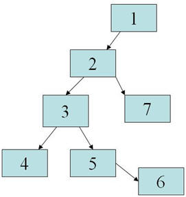
Here we see that step 2 has two children, three and seven, and step 3 has two children, four and five. Step 5 has a lone child, step 6.
Following our rules for preorder traversal, the execution plan steps start at step 4.

Answer: The order of operations is 5, 6, 4, 3, 2, 11, 12, 10, 13, 9, 8, 7, 1.
The Oracle documentation says that the most indented line is the first to be executed, but as we have already noted that not always correct. It's the first indented line required to satisfy the parent step without further requirements.
When a query is run against an Oracle database, Oracle must determine the access path to fetch the required data. It does this by analyzing the requirements of the query and calculating dependencies to return the data requested in a timely fashion. Optimizer statistics are used to choose the most optimal access path, and the final result is returned as an execution plan. The execution plan lists all operations required to satisfy the requirements of the query. This includes table access, index access, joins, filters, sorting, and other operations. The execution plan is ordered based upon the required steps to return the requested data. Two steps on the same indented level are part of the same parent operation. For instance:
1 HASH JOIN
2 TABLE ACCESS FULL TABLE1
3 TABLE ACCESS FULL TABLE2
In the example above, the two full table scans (TABLE ACCESS FULL) are on the same indented level, and are therefore both required to satisfy the parent requirement which is in this case a hash join. Since execution plans are ordered by required operation and ID 1 cannot complete without first completing its indented requirements, the first step to be executed is ID 2 (the table scan on TABLE1) followed by ID 3 (the table scan on TABLE2). Once these are both executed we can execute the HASH JOIN, as all of its requirements have been met. The order of operations is therefore 2, 3, 1.
To read the explain plan, we must start with the first operation and analyze its dependencies in order. Whenever a dependency is met, the parent operation of that dependency is checked to see if all of its requirements are met. In the example above this was very easy because there was only one parent step with two child steps. But what about the example below?
1 HASH JOIN
2 TABLE ACCESS FULL TABLE1
3 TABLE ACCESS BY INDEX ROWID TABLE2
4 INDEX RANGE SCAN TABLE2_IDX
In this case the parent HASH JOIN requires two inputs: a full table scan on TABLE1 and the results of an index access on TABLE2. To read this explain plan, we start at the beginning which is the HASH JOIN. In order to satisfy this join, the first required child step (as noted by indentation) is a full table scan on TABLE1, so the full table scan is executed. The next requirement of the join is an index read on TABLE2; however, this step cannot yet be executed because it has its own dependencies. First an index range scan on TABLE2_IDX is required. This index read satisfies the parent operation which can then be run. Now that the full table scan and indexed table scan are complete, the join operation can complete.
The order of operations here is therefore: 2, 4, 3, 1.
Generally the rule of thumb is that you can start with the most indented operation and start from there. However, this is not always true. The most indented item is simply the deepest child requirement overall. To read an explain plan, we must go down the list of steps from top to bottom and observe each step's requirements. If an operation has requirements (indented operations below it) then those steps are the next to execute. If those steps have further requirements (indented operations below it) then those steps must be executed. Whenever a requirement can be met without further requirements, that operation is completed. Once all required operations under a parent operation are complete, the parent itself can be executed. Consider the below explain plan, a much more complex plan than the previous examples.

So in the example above, the "most indented" rule is only a general rule...it doesn't apply on all complex explain plans. In this example explain plan, there are many steps required in order to return the final query result. Let's look at the order of operations starting at the top:
1. ID 1 SORT ORDER BY - This operation requires one input, which in this case is a HASH GROUP BY (Id 2)
2. ID 2 HASH GROUP BY - This operation requires one input, which in this case is a FILTER (Id 3)
3. ID 3 FILTER - This operation requires one input, which in this case is a HASH JOIN RIGHT OUTER (Id 4)
4. ID 4 HASH JOIN RIGHT OUTER - This operation is a join and requires two inputs. The inputs for this operation are TABLE ACCESS FULL of DIM_E (Id 5) and a HASH JOIN RIGHT OUTER (Id 6)
5. ID 5 TABLE ACCESS FULL -This operation requires no additional input and is required to satisfy the parent operation. This operation is executed. ID 5 COMPLETE
6. ID 6 HASH JOIN RIGHT OUTER - This operation is a join and requires two inputs. The inputs for this operation are TABLE ACCESS FULL of DIM_D (Id 7) and a HASH JOIN (Id 8)
7. ID 7 TABLE ACCESS FULL - This operation requires no additional input and is required to satisfy the parent operation. This operation is executed. ID 7 COMPLETE
8. ID 8 HASH JOIN - This is a join operation requiring two inputs. The inputs for this operation are TABLE ACCESS BY INDEX ROWID of DIM_C (Id 9) and TABLE ACCESS FULL of FACT (Id 16)
9. ID 9 TABLE ACCESS BY INDEX ROWID - This operation requires one input, which in this case is a NESTED LOOP (Id 10)
10. ID 10 NESTED LOOPS - This operation is a join and requires two inputs. The inputs for this operation are another NESTED LOOP (Id 11) and an INDEX RANGE SCAN (id 15)
11. ID 11 NESTED LOOPS - This operation is a join and requires two inputs. The inputs for this operation are TABLE ACCESS FULL of DIM_A (Id 12) and TABLE ACCESS BY INDEX ROWID on DIM_B (Id 13)
12. ID 12 TABLE ACCESS FULL - This operation requires no additional input and is required to satisfy the parent operation. This operation is executed. ID 12 COMPLETE
13. ID 13 TABLE ACCESS BY INDEX ROWID - This operation is a table read based on an index result and requires one input, which in this case is an INDEX RANGE SCAN on IDX_DIM_B_1 (Id 14)
14. ID 14 INDEX RANGE SCAN - This operation requires no additional input and is required to satisfy the parent operation. This operation is executed. ID 14 COMPLETE
Now that we have gone all the way to the most indented child operation, we can start going backwards to see which parent operations have been satisfied.
15. The completion of ID 14 satisfies all input requirements for ID 13. ID 13 is executed. ID 13 COMPLETE
16. The completion of IDs 12 and 13 satisfy all requirements for ID 11. ID 11 is executed. ID 11 COMPLETE
17. ID 11 is now complete, but ID 10 still requires ID 15 to be executed.
18. ID 15 is an INDEX RANGE SCAN on IDX_DIM_C_1 and requires no additional input. The operation is executed. ID 15 COMPLETE
19. Now that ID 11 and 15 are complete, ID 10 has all required inputs to continue and is executed. ID 10 COMPLETE
20. The completion of ID 10 satisfies the only input requirement of ID 9 which is executed. ID 9 COMPLETE
21. The completion of ID 9 satisfies one of two requirements for the HASH JOIN in ID 8. However, ID 16 is still required.
22. ID 16 is a TABLE ACCESS FULL on FACT and requires no additional input. The operation is executed. ID 16 COMPLETE
23. Now that IDs 9 and 16 are complete, ID 8 requires no additional input and is executed. ID 8 COMPLETE
24. ID 7 was already complete and ID 8 is now complete, so all requirements of ID 6 are now complete. ID 6 is executed. ID 6 COMPLETE
25. ID 5 was already complete and ID 6 is now complete, so all requirements of ID 4 are now complete. ID 4 is executed. ID 4 COMPLETE
26. ID 4 was the only required input of ID 3. Since ID 4 is complete, ID 3 is executed. ID 3 COMPLETE
27. ID 3 was the only required input of ID 2. Since ID 3 is complete, ID 2 is executed. ID 2 COMPLETE
28. ID 2 was the only required input of ID 1. Since ID 2 is complete, ID 1 is executed. ID 1 COMPLETE
29. Results of the final step are the final output of the execution plan.
The final order of operations by ID is: 5, 7, 12, 14, 13, 11, 15, 10, 9, 16, 8, 6, 4, 3, 2, 1
A simpler example is this:
1 SELECT
2 NESTED LOOP
3 TABLE ACCESS FULL (TABLE1)
4 TABLE ACCESS BY INDEX ROWID (TABLE2)
5 INDEX RANGE SCAN (TABLE2_IDX)
Even though 5 is the most indented, it is not first. 3 is first because it is the first indented step which satisfies a parent step yet has no further requirements (children)
The order of this one is 3, 5, 4, 2, 1
==============
OPERATION and OPTIONS Values Produced by EXPLAIN PLAN
| Operation | Option | Description |
|---|---|---|
| AND-EQUAL | . | Operation accepting multiple sets of rowids, returning the intersection of the sets, eliminating duplicates. Used for the single-column indexes access path. |
| BITMAP | CONVERSION | TO ROWIDS converts bitmap representations to actual rowids that can be used to access the table. FROM ROWIDS converts the rowids to a bitmap representation. COUNT returns the number of rowids if the actual values are not needed. |
| BITMAP | INDEX | SINGLE VALUE looks up the bitmap for a single key value in the index. RANGE SCAN retrieves bitmaps for a key value range. FULL SCAN performs a full scan of a bitmap index if there is no start or stop key. |
| BITMAP | MERGE | Merges several bitmaps resulting from a range scan into one bitmap. |
| BITMAP | MINUS | Subtracts bits of one bitmap from another. Row source is used for negated predicates. Can be used only if there are nonnegated predicates yielding a bitmap from which the subtraction can take place. An example appears in "Viewing Bitmap Indexes with EXPLAIN PLAN". |
| BITMAP | OR | Computes the bitwise OR of two bitmaps. |
| BITMAP | AND | Computes the bitwise AND of two bitmaps. |
| BITMAP | KEY ITERATION | Takes each row from a table row source and finds the corresponding bitmap from a bitmap index. This set of bitmaps are then merged into one bitmap in a following BITMAP MERGE operation. |
| CONNECT BY | . | Retrieves rows in hierarchical order for a query containing a CONNECT BY clause. |
| CONCATENATION | . | Operation accepting multiple sets of rows returning the union-all of the sets. |
| COUNT | . | Operation counting the number of rows selected from a table. |
| COUNT | STOPKEY | Count operation where the number of rows returned is limited by the ROWNUM expression in theWHERE clause. |
| CUBE SCAN | . | Uses inner joins for all cube access. |
| CUBE SCAN | PARTIAL OUTER | Uses an outer join for at least one dimension, and inner joins for the other dimensions. |
| CUBE SCAN | OUTER | Uses outer joins for all cube access. |
| DOMAIN INDEX | . | Retrieval of one or more rowids from a domain index. The options column contain information supplied by a user-defined domain index cost function, if any. |
| FILTER | . | Operation accepting a set of rows, eliminates some of them, and returns the rest. |
| FIRST ROW | . | Retrieval of only the first row selected by a query. |
| FOR UPDATE | . | Operation retrieving and locking the rows selected by a query containing a FOR UPDATE clause. |
| HASH | GROUP BY | Operation hashing a set of rows into groups for a query with a GROUP BY clause. |
| HASH | GROUP BY PIVOT | Operation hashing a set of rows into groups for a query with a GROUP BY clause. The PIVOT option indicates a pivot-specific optimization for the HASH GROUP BY operator. |
| HASH JOIN (These are join operations.) | . | Operation joining two sets of rows and returning the result. This join method is useful for joining large data sets of data (DSS, Batch). The join condition is an efficient way of accessing the second table. Query optimizer uses the smaller of the two tables/data sources to build a hash table on the join key in memory. Then it scans the larger table, probing the hash table to find the joined rows. |
| HASH JOIN | ANTI | Hash (left) antijoin |
| HASH JOIN | SEMI | Hash (left) semijoin |
| HASH JOIN | RIGHT ANTI | Hash right antijoin |
| HASH JOIN | RIGHT SEMI | Hash right semijoin |
| HASH JOIN | OUTER | Hash (left) outer join |
| HASH JOIN | RIGHT OUTER | Hash right outer join |
| INDEX (These are access methods.) | UNIQUE SCAN | Retrieval of a single rowid from an index. |
| INDEX | RANGE SCAN | Retrieval of one or more rowids from an index. Indexed values are scanned in ascending order. |
| INDEX | RANGE SCAN DESCENDING | Retrieval of one or more rowids from an index. Indexed values are scanned in descending order. |
| INDEX | FULL SCAN | Retrieval of all rowids from an index when there is no start or stop key. Indexed values are scanned in ascending order. |
| INDEX | FULL SCAN DESCENDING | Retrieval of all rowids from an index when there is no start or stop key. Indexed values are scanned in descending order. |
| INDEX | FAST FULL SCAN | Retrieval of all rowids (and column values) using multiblock reads. No sorting order can be defined. Compares to a full table scan on only the indexed columns. Only available with the cost based optimizer. The index must contain all the columns referenced in the query. |
| INDEX | SKIP SCAN | Retrieval of rowids from a concatenated index without using the leading column(s) in the index. Introduced in Oracle9i. Only available with the cost based optimizer. Index skip scans improve index scans by non-prefix columns since it is often faster to scan index blocks than scanning table data blocks. A non-prefix index is an index which does not contain a key column as its first column. |
| INLIST ITERATOR | . | Iterates over the next operation in the plan for each value in the IN-list predicate. |
| INTERSECTION | . | Operation accepting two sets of rows and returning the intersection of the sets, eliminating duplicates. |
| MERGE JOIN (These are join operations.) | . | Operation accepting two sets of rows, each sorted by a specific value, combining each row from one set with the matching rows from the other, and returning the result. |
| MERGE JOIN | OUTER | Merge join operation to perform an outer join statement. |
| MERGE JOIN | ANTI | Merge antijoin. |
| MERGE JOIN | SEMI | Merge semijoin. |
| MERGE JOIN | CARTESIAN | Can result from 1 or more of the tables not having any join conditions to any other tables in the statement. Can occur even with a join and it may not be flagged as CARTESIAN in the plan. |
| CONNECT BY | . | Retrieval of rows in hierarchical order for a query containing a CONNECT BY clause. |
| MAT_VIEW REWITE ACCESS (These are access methods.) | FULL | Retrieval of all rows from a materialized view. |
| MAT_VIEW REWITE ACCESS | SAMPLE | Retrieval of sampled rows from a materialized view. |
| MAT_VIEW REWITE ACCESS | CLUSTER | Retrieval of rows from a materialized view based on a value of an indexed cluster key. |
| MAT_VIEW REWITE ACCESS | HASH | Retrieval of rows from materialized view based on hash cluster key value. |
| MAT_VIEW REWITE ACCESS | BY ROWID RANGE | Retrieval of rows from a materialized view based on a rowid range. |
| MAT_VIEW REWITE ACCESS | SAMPLE BY ROWID RANGE | Retrieval of sampled rows from a materialized view based on a rowid range. |
| MAT_VIEW REWITE ACCESS | BY USER ROWID | If the materialized view rows are located using user-supplied rowids. |
| MAT_VIEW REWITE ACCESS | BY INDEX ROWID | If the materialized view is nonpartitioned and rows are located using index(es). |
| MAT_VIEW REWITE ACCESS | BY GLOBAL INDEX ROWID | If the materialized view is partitioned and rows are located using only global indexes. |
| MAT_VIEW REWITE ACCESS | BY LOCAL INDEX ROWID | If the materialized view is partitioned and rows are located using one or more local indexes and possibly some global indexes. Partition Boundaries: The partition boundaries might have been computed by: A previous PARTITION step, in which case the PARTITION_START and PARTITION_STOP column values replicate the values present in the PARTITIONstep, and the PARTITION_ID contains the ID of the PARTITION step. Possible values for PARTITION_START and PARTITION_STOP are NUMBER(n),KEY, INVALID. The MAT_VIEW REWRITE ACCESS or INDEX step itself, in which case the PARTITION_ID contains theID of the step. Possible values for PARTITION_START and PARTITION_STOP are NUMBER(n), KEY,ROW REMOVE_LOCATION (MAT_VIEW REWRITE ACCESS only), and INVALID. |
| MINUS | . | Operation accepting two sets of rows and returning rows appearing in the first set but not in the second, eliminating duplicates. |
| NESTED LOOPS (These are join operations.) | . | Operation accepting two sets of rows, an outer set and an inner set. Oracle compares each row of the outer set with each row of the inner set, returning rows that satisfy a condition. This join method is useful for joining small subsets of data (OLTP). The join condition is an efficient way of accessing the second table. |
| NESTED LOOPS | OUTER | Nested loops operation to perform an outer join statement. |
| PARTITION | . | Iterates over the next operation in the plan for each partition in the range given by thePARTITION_START and PARTITION_STOP columns. PARTITIONdescribes partition boundaries applicable to a single partitioned object (table or index) or to a set of equi-partitioned objects (a partitioned table and its local indexes). The partition boundaries are provided by the values ofPARTITION_START and PARTITION_STOP of the PARTITION. |
| PARTITION | SINGLE | Access one partition. |
| PARTITION | ITERATOR | Access many partitions (a subset). |
| PARTITION | ALL | Access all partitions. |
| PARTITION | INLIST | Similar to iterator, but based on an IN-list predicate. |
| PARTITION | INVALID | Indicates that the partition set to be accessed is empty. |
| PX ITERATOR | BLOCK, CHUNK | Implements the division of an object into block or chunk ranges among a set of parallel slaves |
| PX COORDINATOR | . | Implements the Query Coordinator which controls, schedules, and executes the parallel plan below it using parallel query slaves. It also represents a serialization point, as the end of the part of the plan executed in parallel and always has a PX SEND QC operation below it. |
| PX PARTITION | . | Same semantics as the regular PARTITION operation except that it appears in a parallel plan |
| PX RECEIVE | . | Shows the consumer/receiver slave node reading repartitioned data from a send/producer (QC or slave) executing on a PX SEND node. This information was formerly displayed into theDISTRIBUTION column. |
| PX SEND | QC (RANDOM), HASH, RANGE | Implements the distribution method taking place between two parallel set of slaves. Shows the boundary between two slave sets and how data is repartitioned on the send/producer side (QC or side. This information was formerly displayed into the DISTRIBUTION column. |
| REMOTE | . | Retrieval of data from a remote database. |
| SEQUENCE | . | Operation involving accessing values of a sequence. |
| SORT | AGGREGATE | Retrieval of a single row that is the result of applying a group function to a group of selected rows. |
| SORT | UNIQUE | Operation sorting a set of rows to eliminate duplicates. |
| SORT | GROUP BY | Operation sorting a set of rows into groups for a query with a GROUP BY clause. |
| SORT | GROUP BY PIVOT | Operation sorting a set of rows into groups for a query with a GROUP BY clause. The PIVOT option indicates a pivot-specific optimization for the SORT GROUP BY operator. |
| SORT | JOIN | Operation sorting a set of rows before a merge-join. |
| SORT | ORDER BY | Operation sorting a set of rows for a query with an ORDER BY clause. |
| TABLE ACCESS (These are access methods.) | FULL | Retrieval of all rows from a table. |
| TABLE ACCESS | SAMPLE | Retrieval of sampled rows from a table. |
| TABLE ACCESS | CLUSTER | Retrieval of rows from a table based on a value of an indexed cluster key. |
| TABLE ACCESS | HASH | Retrieval of rows from table based on hash cluster key value. |
| TABLE ACCESS | BY ROWID RANGE | Retrieval of rows from a table based on a rowid range. |
| TABLE ACCESS | SAMPLE BY ROWID RANGE | Retrieval of sampled rows from a table based on a rowid range. |
| TABLE ACCESS | BY USER ROWID | If the table rows are located using user-supplied rowids. |
| TABLE ACCESS | BY INDEX ROWID | If the table is nonpartitioned and rows are located using index(es). |
| TABLE ACCESS | BY GLOBAL INDEX ROWID | If the table is partitioned and rows are located using only global indexes. |
| TABLE ACCESS | BY LOCAL INDEX ROWID | If the table is partitioned and rows are located using one or more local indexes and possibly some global indexes. Partition Boundaries: The partition boundaries might have been computed by: A previous PARTITION step, in which case the PARTITION_START and PARTITION_STOP column values replicate the values present in the PARTITIONstep, and the PARTITION_ID contains the ID of the PARTITION step. Possible values for PARTITION_START and PARTITION_STOP are NUMBER(n),KEY, INVALID. The TABLE ACCESS or INDEX step itself, in which case the PARTITION_ID contains the ID of the step. Possible values for PARTITION_START and PARTITION_STOP are NUMBER(n), KEY, ROWREMOVE_LOCATION (TABLE ACCESS only), and INVALID. |
| TRANSPOSE | . | Operation evaluating a PIVOT operation by transposing the results of GROUP BY to produce the final pivoted data. |
| UNION | . | Operation accepting two sets of rows and returns the union of the sets, eliminating duplicates. |
| UNPIVOT | . | Operation that rotates data from columns into rows. |
| VIEW | . | Operation performing a view's query and then returning the resulting rows to another operation. |
Nested Loop - As a rule of thumb, if a query returns less than 10% of the rows from the tables involved, you should be using nested loops. Use hash joins or sort merges if 10% or more of the rows are being returned. A nested loop join involves the designation of one table as the driving table (also called the outer table) in the join loop. The other table in the join is called the inner table. Oracle fetches all the rows of the inner table for every row in the driving table.
Hash Join - To perform a hash join, a hash table is created in the memory of the smallest table, and then the other table is scanned. The rows from the second table are compared to the hash. A hash join will usually run faster than a merge join (involving a sort, then a merge) if memory is adequate to hold the entire table that is being hashed. The entire result set must be determined before. For starters, a hash join can only be used for joins based on equality (=), and not for joins based on ranges (<, <=, >, >=). If I have a WHERE clause on the join columns such as WHERE o.owner <= w.owner, a hash join will not work.
Merge joins - The sort join operation sorts the inputs on the join key, and the merge join operation merges the sorted lists . Merge Joins will work effectively for joins based on equality as well as for those based on ranges. In addition, merge joins will often run faster when all of the columns in the WHERE clause are pre-sorted by being in an index. In this case, the rows are simply plucked from the tables using the ROWID in the index.
With a merge join, all tables are sorted, unless all of the columns in the WHERE clause are contained within an index. This sort can be expensive, and it explains why a hash join will often run faster than a merge join. As with a hash join, the entire result set must be determined before a single row is returned to the user. Therefore, merge and hash joins are usually used for reporting and batch processing.
Monitoring Adaptive Cursor Sharing
The V$SQL view contains two columns, named IS_BIND_SENSITIVE and IS_BIND_AWARE, that help you monitor adaptive cursor sharing in the database. The IS_BIND_SENSITIVE column lets you know whether a cursor is bind sensitive, and the IS_BIND_AWARE column shows whether the database has marked a cursor for bind-aware cursor sharing. The following query, for example, tells you which SQL statements are binds sensitive or bind aware:
SQL> SELECT sql_id, executions, is_bind_sensitive, is_bind_aware FROM v$sql;
SQL_ID EXECUTIONS I I
-------------- ----------- --- ---
57pfs5p8xc07w 21 Y N
1gfaj4z5hn1kf 4 Y N
1gfaj4z5hn1kf 4 N N
...
294 rows selected.
SQL>
In this query, the IS_BIND_SENSITIVE column shows whether the database will generate different execution plans based on bind variable values. Any cursor that shows an IS_BIND_SENSITIVE column value of Y is a candidate for an execution plan change. When the database plans to use multiple execution plans for a statement based on the observed values of the bind variables, it marks the IS_BIND_AWARE column Y for that statement. This means that the optimizer realizes that different bind variable values would lead to different data patterns, which requires the statement to be hardparsed during the next execution. In order to decide whether to change the execution plan, the database evaluates the next few executions of the SQL statement. If the database decides to change a statement’s execution plan, it marks the cursor bind aware and puts a value of Y in the IS_BIND_AWARE column for that statement. A bind-aware cursor is one for which the database has actually modified the execution plan based on the observed values of the bind variables.
You can use the following views to manage the adaptive cursor sharing feature:
• V$SQL_CS_HISTOGRAM: Shows the distribution of the execution count across the execution history histogram
• V$SQL_CS_SELECTIVITY: Shows the selectivity ranges stored in cursors for predicates with bind variables
• V$SQL_CS_STATISTICS: Contains the execution statistics of a cursor using different bind sets gathered by the database

No comments:
Post a Comment